ggplot2 Quick Reference: colour (and fill)
Specifying Colours
In R, a colour is represented as a string (see Color Specification section of the R par() function). Basically, a colour is defined, like in HTML/CSS, using the hexadecimal values (00 to FF) for red, green, and blue, concatenated into a string, prefixed with a "#". A pure red colour this is represented with "#FF0000".
Predefined Colour Names
Besides the "#RRGGBB" RGB colour strings, one can also use one of R's predefined named colours:
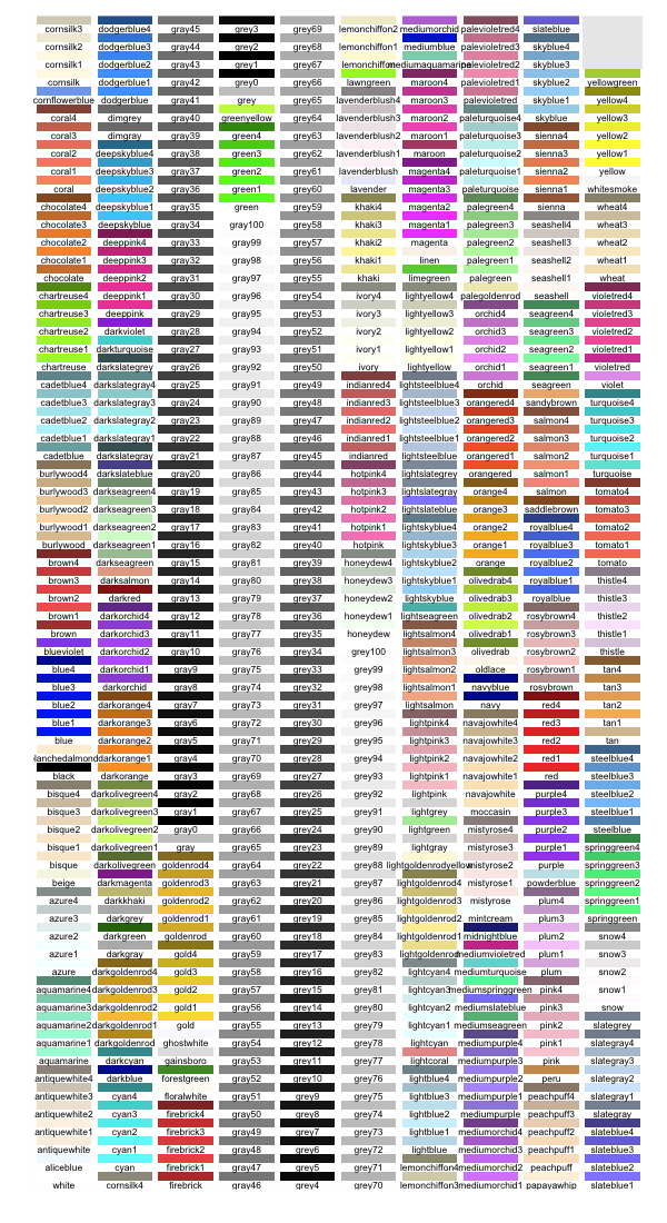
d=data.frame(c=colors(), y=seq(0, length(colors())-1)%%66, x=seq(0, length(colors())-1)%/%66)
ggplot() +
scale_x_continuous(name="", breaks=NA, expand=c(0, 0)) +
scale_y_continuous(name="", breaks=NA, expand=c(0, 0)) +
scale_fill_identity() +
geom_rect(data=d, mapping=aes(xmin=x, xmax=x+1, ymin=y, ymax=y+1), fill="white") +
geom_rect(data=d, mapping=aes(xmin=x+0.05, xmax=x+0.95, ymin=y+0.5, ymax=y+1, fill=c)) +
geom_text(data=d, mapping=aes(x=x+0.5, y=y+0.5, label=c), colour="black", hjust=0.5, vjust=1, size=3)
Hue Saturation Value (HSV) = Hue Saturation Brightness (HSB) Colour Space
A colour can be specified using R's hsv() function that takes three arguments: hue, saturation, and value (brightness), all in the range [0, 1].
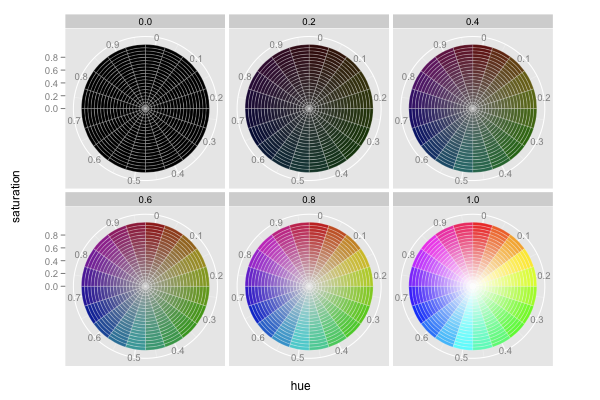
d=expand.grid(h=seq(0,0.95,0.05), s=seq(0,0.95,0.05), v=seq(0,1,0.2))
ggplot() +
coord_polar(theta="x") +
facet_wrap(~v) +
scale_x_continuous(name="hue", limits=c(0,1), breaks=seq(0.025,0.925,0.1), labels=seq(0,0.9,0.1)) +
scale_y_continuous(name="saturation", breaks=seq(0, 1, 0.2)) +
scale_fill_identity() +
geom_rect(data=d, mapping=aes(xmin=h, xmax=h+resolution(h), ymin=s, ymax=s+resolution(s), fill=hsv(h,s,v)), color="white", size=0.1)
Hue Chroma Luminance (HCL) Colour Space
A colour can be specified using R's hcl() function that takes three arguments: hue [0,360], chroma [0,100], and luminance [0,100]. This space is similar to the HSV space, however, in the HCL space steps of equal size correspond to approximately equal perceptual changes in colour. Note that the possible values of chroma and luminance actually depend on the specific hue. The ranges above are only indicative.
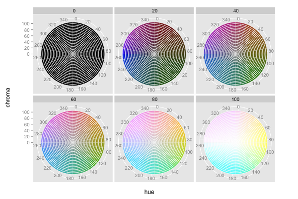
d=expand.grid(h=seq(0,350,10), c=seq(0,100,5), l=seq(0,100,20))
ggplot() +
coord_polar(theta="x")+facet_wrap(~l) +
scale_x_continuous(name="hue", limits=c(0,360), breaks=seq(5,345,20), labels=seq(0,340,20)) +
scale_y_continuous(name="chroma", breaks=seq(0, 100, 20)) +
scale_fill_identity() +
geom_rect(data=d, mapping=aes(xmin=h, xmax=h+resolution(h), ymin=c, ymax=c+resolution(c), fill=hcl(h,c,l)), color="white", size=0.1)
Red Green Blue (RGB) Colour Space
RGB is the built-in colour space. Instead of "manually" creating a #RRGGBB colour string, a colour can be specified using R's rgb() function that takes three arguments: red, green, and blue (which, by default, all have a range of [0, 1]).
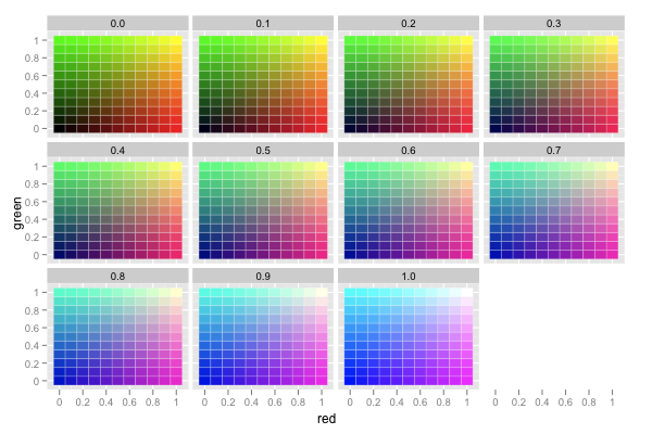
d=expand.grid(r=seq(0,1,0.1), g=seq(0,1,0.1), b=seq(0,1,0.1))
ggplot() +
facet_wrap(~b) +
scale_x_continuous(name="red", breaks=seq(0.05, 1.05, 0.2), labels=seq(0, 1, 0.2)) +
scale_y_continuous(name="green", breaks=seq(0.05, 1.05, 0.2), labels=seq(0, 1, 0.2)) +
scale_fill_identity() +
geom_rect(data=d, mapping=aes(xmin=r, xmax=r+resolution(r), ymin=g, ymax=g+resolution(g), fill=rgb(r,g,b)), color="white", size=0.1)
For best visual performance, we recommend mapping data onto the hue of a colour (using the HSV or HCL colour spaces).
Publication Highlights
OOPSLA'15 - Use at Own Risk
PPPJ'13 - Jikes RVM Debugger
PLDI'12 - Algorithmic Profiling
OOPSLA'11 - Catch Me
ECOOP'11 - Beauty and Beast
PLDI'10 - Profiler (In)Accuracy
ASPLOS'09 - Measurement Bias
More...
Blast
Our framework for bytecode-level information-flow tracing of Java programs.

Jikes RDB
Working with the Jikes RVM? Use Jikes RDB for debugging your VM hacks.

Now built on top of LLDB, so it works on OS X and on Linux.