ggplot2 Quick Reference: coord
The coordinate system of a plot, together with the x and y position scale, determines the location of geoms.
- coord_cartesian - (default) cartesian coordinate system (x horizontal from left to right, y vertical from bottom to top)
- coord_flip - flipped cartesian coordinate system (x vertical from bottom to top, y horizontal from left to right)
- coord_trans
- coord_equal
- coord_polar - polar coordinate system; the x (or y) scale is mapped to the angle (theta)
- coord_map - various map projections
Example
Assume the following data frame:
d=data.frame(height=c(1,2,2,3,4), weight=c(1,3,4,4,2))
And assume the following plot:
p = ggplot() +
geom_line(data=d, mapping=aes(x=height, y=weight)) +
geom_point(data=d, mapping=aes(x=height, y=weight), size=8, fill="white", shape=21) +
geom_text(data=d,mapping=aes(x=height, y=weight, label=seq(1,nrow(d))))
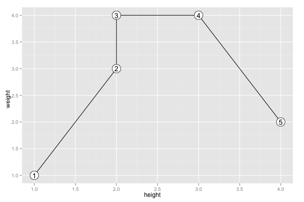
coord_cartesian
p + coord_cartesian()
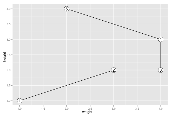
coord_flip
p + coord_flip()
coord_trans
p + coord_trans(xtrans="log10", ytrans="log10")
![]()
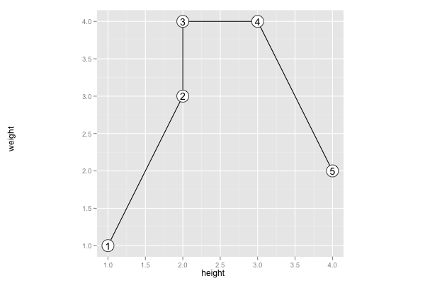
coord_equal
p + coord_equal()
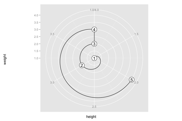
coord_polar
p + coord_polar(theta="x")
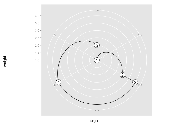
p + coord_polar(theta="y")
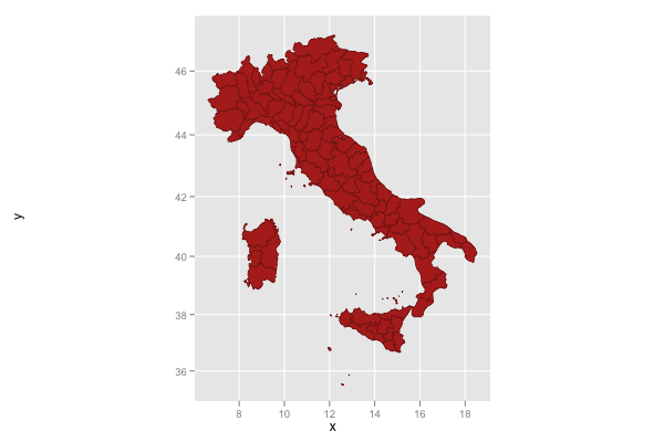
Example with coord_map
Load the "maps" package and create a data frame containing the latitudes and longitudes of the map of Italy.
require(maps)
d = data.frame(map(database="italy", plot=F)[c("x", "y")])
Create a plot using coord_map with its default (mercator) projection:
ggplot() +
coord_map() +
geom_polygon(data=d, mapping=aes(x=x, y=y), fill=hsv(0, 1, 0.7), color=hsv(0, 1, 0.5), size=0.2)
Publication Highlights
OOPSLA'15 - Use at Own Risk
PPPJ'13 - Jikes RVM Debugger
PLDI'12 - Algorithmic Profiling
OOPSLA'11 - Catch Me
ECOOP'11 - Beauty and Beast
PLDI'10 - Profiler (In)Accuracy
ASPLOS'09 - Measurement Bias
More...
Blast
Our framework for bytecode-level information-flow tracing of Java programs.

Jikes RDB
Working with the Jikes RVM? Use Jikes RDB for debugging your VM hacks.

Now built on top of LLDB, so it works on OS X and on Linux.