ggplot2 Quick Reference: facet
The faceting approach supported by ggplot2 partitions a plot into a matrix of panels. Each panel shows a different subset of the data. There are two faceting approaches:
- facet_wrap(~cell) - univariate: create a 1-d strip of panels, based on one factor, and wrap the strip into a 2-d matrix
- facet_grid(row~col) - (usually) bivariate: create a 2-d matrix of panels, based on two factors
Example Data
Let's generate some data that could be the result of a hypothetical experiment to evaluate the benefits of a performance optimization in a virtual machine. The virtual machine can be configured to use various garbage collection algorithms (column "gc" in our data frame) and to use different heap sizes (column "heapSize"). We measure the run time of a set of benchmark applications (column "benchmark"). We collect ten observations (column "obs") for each benchmark on each garbage collector with each heap size.
d=expand.grid(obs=0:10, benchmark=c('antlr', 'bloat', 'chart', 'eclipse', 'fop', 'hsqldb', 'jython', 'luindex', 'lusearch', 'pmd', 'xalan'), gc=c('CopyMS', 'GenCopy', 'GenImmix', 'GenMS', 'Immix'), opt=c('on', 'off'), heapSize=seq(from=1.5, to=4, by=0.5))
d$time = rexp(nrow(d), 0.01)+1000
d$time = d$time + abs(d$heapSize-3)*100
d$time[d$opt=='on'] = d$time[d$opt=='on']-200

d$time[d$opt=='on' & d$benchmark=='bloat'] = d$time[d$opt=='on' & d$benchmark=='bloat'] + 190
d$time[d$opt=='on' & d$benchmark=='pmd' & d$gc=='Immix'] = d$time[d$opt=='on' & d$benchmark=='pmd' & d$gc=='Immix'] + 600
No Faceting
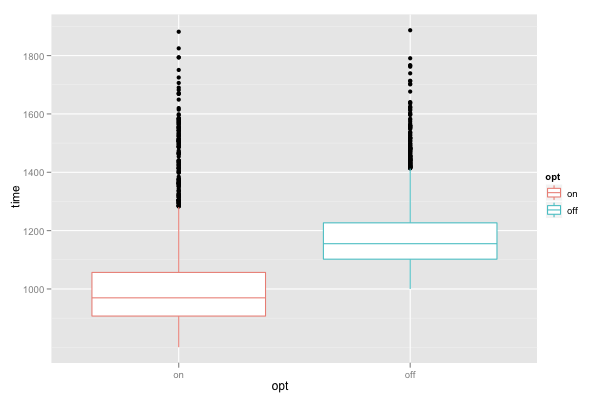
First, let's create a very high level summarization of that data:
ggplot() +
geom_boxplot(data=d, mapping=aes(x=opt, y=time, color=opt))
facet_wrap()
Now let's use faceting to break the results down by benchmark:
ggplot() +
facet_wrap(~benchmark) +
geom_boxplot(data=d, mapping=aes(x=opt, y=time, color=opt))
facet_wrap(~benchmark) creates a separate panel for each benchmark. The panels are wrapped into multiple rows on a grid. Wrapping the panels is especially useful when we have a factor with a larger number of levels (such as benchmarks, which has 11 levels); without wrapping, the plot can become overly wide (or the individual panels overly narrow).
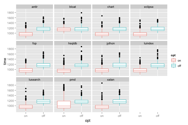
The above plot shows that the "bloat" benchmark does not seem to benefit much from our optimization (its run time does not decrease much when we enable the optimization). The plot also shows that the optimized run time of the "pmd" benchmark is dispersed more (the box is taller).
facet_grid()
And now let's facet by two variables: in addition to benchmark (horizontally), we also use gc (vertically):
ggplot() +
facet_grid(gc~benchmark) +
geom_boxplot(data=d, mapping=aes(x=opt, y=time, color=opt))
facet_grid(gc~benchmark) produces a separate panel for each gc-benchmark combination and places the panels in a grid with one row for each gc and one column for each benchmark.
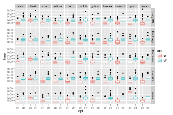
The above plot shows the reason for the wider dispersion of the time for the "pmd" benchmark: for most gcs, switching on the optimization reduces run time, however, when running on the "Immix" collector, the optimization actually degrades performance (increases run time).
Publication Highlights
OOPSLA'15 - Use at Own Risk
PPPJ'13 - Jikes RVM Debugger
PLDI'12 - Algorithmic Profiling
OOPSLA'11 - Catch Me
ECOOP'11 - Beauty and Beast
PLDI'10 - Profiler (In)Accuracy
ASPLOS'09 - Measurement Bias
More...
Blast
Our framework for bytecode-level information-flow tracing of Java programs.

Jikes RDB
Working with the Jikes RVM? Use Jikes RDB for debugging your VM hacks.

Now built on top of LLDB, so it works on OS X and on Linux.