ggplot2 Quick Reference: Themes
")
")


A plot can be themed by adding a theme. ggplot2 provides two built-in themes:
- theme_grey() - the default theme, with a grey background
- theme_bw() - a theme with a white background
To be more precise, ggplot2 provides functions that create a theme. These functions can be used to add a specific theme to a plot:
ggplot() + ... + theme_bw()
The theme produced by such a function is simply a structure containing a list of options. These options describe the visual properties of the axes, legends, panels, strips, and the overall plot. Note that these options define everything but the layers contained in the plot. If you create a layer to draw red dots and blue lines, the theme will not change these settings.
When adding a theme to a plot, you can override some of the theme's options with opts(...). The example below uses theme_grey() for the plot, but overrides legend.background to fill the legend's space with a very light grey (theme_grey sets the legend fill to white otherwise).
ggplot() + ... + theme_grey() + opts(legend.background = theme_rect(fill="grey95", colour=NA))
When using opts() and adding a theme (like in the command right above), make sure that you add the theme before overriding the options (otherwise the opts(...) has no effect).
The Currently Selected Theme
If you are not explicitly adding a theme to a plot, ggplot2 uses the currently selected theme. At startup, ggplot2 selects theme_grey(). You can change the current selection with theme_set(...), you can access the currently selected theme with theme_get(), and you can even modify the properties of the currently selected theme with theme_update(...).
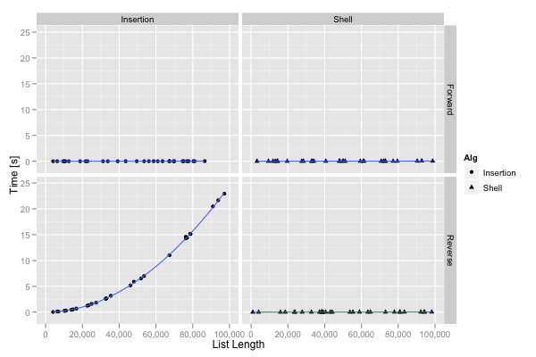
theme_grey()
The theme_grey() function creates the default theme of ggplot2. Here is an example plot using this theme:
Here is its definition, straight from ggplot2's source code:
theme_gray <- function(base_size = 12) {
  structure(list(
    axis.line =         theme_blank(),
    axis.text.x =       theme_text(size = base_size * 0.8 , lineheight = 0.9, colour = "grey50", vjust = 1),
    axis.text.y =       theme_text(size = base_size * 0.8, lineheight = 0.9, colour = "grey50", hjust = 1),
    axis.ticks =        theme_segment(colour = "grey50"),
    axis.title.x =      theme_text(size = base_size, vjust = 0.5),
    axis.title.y =      theme_text(size = base_size, angle = 90, vjust = 0.5),
    axis.ticks.length = unit(0.15, "cm"),
    axis.ticks.margin = unit(0.1, "cm"),

    legend.background = theme_rect(colour="white"),
    legend.key =        theme_rect(fill = "grey95", colour = "white"),
    legend.key.size =   unit(1.2, "lines"),
    legend.text =       theme_text(size = base_size * 0.8),
    legend.title =      theme_text(size = base_size * 0.8, face = "bold", hjust = 0),
    legend.position =   "right",

    panel.background =  theme_rect(fill = "grey90", colour = NA),
    panel.border =      theme_blank(),
    panel.grid.major =  theme_line(colour = "white"),
    panel.grid.minor =  theme_line(colour = "grey95", size = 0.25),
    panel.margin =      unit(0.25, "lines"),

    strip.background =  theme_rect(fill = "grey80", colour = NA),
    strip.text.x =      theme_text(size = base_size * 0.8),
    strip.text.y =      theme_text(size = base_size * 0.8, angle = -90),

    plot.background =   theme_rect(colour = NA, fill = "white"),
    plot.title =        theme_text(size = base_size * 1.2),
    plot.margin =       unit(c(1, 1, 0.5, 0.5), "lines")
  ), class = "options")
}
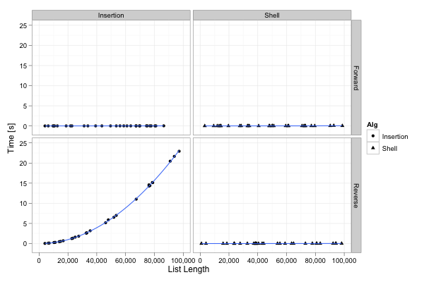
theme_bw()
The theme_bw() function produces a mostly (but not entirely) black-and-white theme.
This is the definition of theme_bw() straight from ggplot2's source code:
theme_bw <- function(base_size = 12) {
  structure(list(
    axis.line =         theme_blank(),
    axis.text.x =       theme_text(size = base_size * 0.8 , lineheight = 0.9, vjust = 1),
    axis.text.y =       theme_text(size = base_size * 0.8, lineheight = 0.9, hjust = 1),
    axis.ticks =        theme_segment(colour = "black", size = 0.2),
    axis.title.x =      theme_text(size = base_size, vjust = 1),
    axis.title.y =      theme_text(size = base_size, angle = 90, vjust = 0.5),
    axis.ticks.length = unit(0.3, "lines"),
    axis.ticks.margin = unit(0.5, "lines"),

    legend.background = theme_rect(colour=NA),
    legend.key =        theme_rect(colour = "grey80"),
    legend.key.size =   unit(1.2, "lines"),
    legend.text =       theme_text(size = base_size * 0.8),
    legend.title =      theme_text(size = base_size * 0.8, face = "bold", hjust = 0),
    legend.position =   "right",

    panel.background =  theme_rect(fill = "white", colour = NA),
    panel.border =      theme_rect(fill = NA, colour="grey50"),
    panel.grid.major =  theme_line(colour = "grey90", size = 0.2),
    panel.grid.minor =  theme_line(colour = "grey98", size = 0.5),
    panel.margin =      unit(0.25, "lines"),

    strip.background =  theme_rect(fill = "grey80", colour = "grey50"),
    strip.text.x =      theme_text(size = base_size * 0.8),
    strip.text.y =      theme_text(size = base_size * 0.8, angle = -90),

    plot.background =   theme_rect(colour = NA),
    plot.title =        theme_text(size = base_size * 1.2),
    plot.margin =       unit(c(1, 1, 0.5, 0.5), "lines")
  ), class = "options")
}
Creating Your Own Theme
You can easily create your own theme by defining such a function on your own, and then adding it to your plot with ggplot() + ... + myOwnTheme(). Here is a theme where all elements have color=NA and thus are invisible.
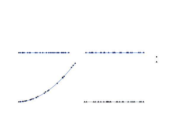
And here is the function creating that theme:
theme_invisible <- function(base_size = 12) {
  structure(list(
    axis.line =         theme_blank(),
    axis.text.x =       theme_text(colour = NA,size = base_size * 0.8 , lineheight = 0.9, vjust = 1),
    axis.text.y =       theme_text(colour = NA,size = base_size * 0.8, lineheight = 0.9, hjust = 1),
    axis.ticks =        theme_segment(colour = NA, size = 0.2),
    axis.title.x =      theme_text(colour = NA,size = base_size, vjust = 1),
    axis.title.y =      theme_text(colour = NA,size = base_size, angle = 90, vjust = 0.5),
    axis.ticks.length = unit(0.3, "lines"),
    axis.ticks.margin = unit(0.5, "lines"),

    legend.background = theme_rect(colour=NA),
    legend.key =        theme_rect(colour = NA, ),
    legend.key.size =   unit(1.2, "lines"),
    legend.text =       theme_text(colour = NA,size = base_size * 0.8),
    legend.title =      theme_text(colour = NA,size = base_size * 0.8, face = "bold", hjust = 0),
    legend.position =   "right",

    panel.background =  theme_rect(fill = NA, colour = NA),
    panel.border =      theme_rect(fill = NA, colour=NA),
    panel.grid.major =  theme_line(colour = NA, size = 0.2),
    panel.grid.minor =  theme_line(colour = NA, size = 0.5),
    panel.margin =      unit(0.25, "lines"),

    strip.background =  theme_rect(fill = NA, colour = NA),
    strip.text.x =      theme_text(colour = NA,size = base_size * 0.8),
    strip.text.y =      theme_text(colour = NA,size = base_size * 0.8, angle = -90),

    plot.background =   theme_rect(colour = NA),
    plot.title =        theme_text(colour = NA,size = base_size * 1.2),
    plot.margin =       unit(c(1, 1, 0.5, 0.5), "lines")
  ), class = "options")
}
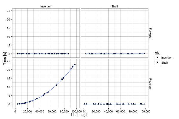
A Truly Black-And-White Theme
The following theme uses only black and white (unlike theme_bw(), which also uses various levels of grey). Only using black and white may be useful when producing plots for black-and-white publications.
Here is the corresponding theme function:
theme_complete_bw <- function(base_size = 12) {
  structure(list(
    axis.line =         theme_blank(),
    axis.text.x =       theme_text(size = base_size * 0.8 , lineheight = 0.9, colour = "black", vjust = 1),
    axis.text.y =       theme_text(size = base_size * 0.8, lineheight = 0.9, colour = "black", hjust = 1),
    axis.ticks =        theme_segment(colour = "black"),
    axis.title.x =      theme_text(size = base_size, vjust = 0.5),
    axis.title.y =      theme_text(size = base_size, angle = 90, vjust = 0.5),
    axis.ticks.length = unit(0.15, "cm"),
    axis.ticks.margin = unit(0.1, "cm"),

    legend.background = theme_rect(colour=NA),
    legend.key =        theme_rect(fill = NA, colour = "black", size = 0.25),
    legend.key.size =   unit(1.2, "lines"),
    legend.text =       theme_text(size = base_size * 0.8),
    legend.title =      theme_text(size = base_size * 0.8, face = "bold", hjust = 0),
    legend.position =   "right",

    panel.background =  theme_rect(fill = NA, colour = "black", size = 0.25),
    panel.border =      theme_blank(),
    panel.grid.major =  theme_line(colour = "black", size = 0.05),
    panel.grid.minor =  theme_line(colour = "black", size = 0.05),
    panel.margin =      unit(0.25, "lines"),

    strip.background =  theme_rect(fill = NA, colour = NA),
    strip.text.x =      theme_text(colour = "black", size = base_size * 0.8),
    strip.text.y =      theme_text(colour = "black", size = base_size * 0.8, angle = -90),

    plot.background =   theme_rect(colour = NA, fill = "white"),
    plot.title =        theme_text(size = base_size * 1.2),
    plot.margin =       unit(c(1, 1, 0.5, 0.5), "lines")
  ), class = "options")
}
Publication Highlights
OOPSLA'15 - Use at Own Risk
PPPJ'13 - Jikes RVM Debugger
PLDI'12 - Algorithmic Profiling
OOPSLA'11 - Catch Me
ECOOP'11 - Beauty and Beast
PLDI'10 - Profiler (In)Accuracy
ASPLOS'09 - Measurement Bias
More...
Blast
Our framework for bytecode-level information-flow tracing of Java programs.

Jikes RDB
Working with the Jikes RVM? Use Jikes RDB for debugging your VM hacks.

Now built on top of LLDB, so it works on OS X and on Linux.